
Principles of Magnetism
Principles of Magnetism and Stray Currents in Rotating Machinery
By Paul I. Nippes, P.E., President of Magnetic Products and Services, Inc.
Introduction
This paper presents a collection of information that should be useful for understanding magnetism in machinery. It can also be used as a reference guide for engineers and technicians regarding the principles of magnetism and how to measure and remove it. Delving briefly into some of the effects of magnetism, such as stray currents. A table is included which shows acceptable levels of magnetism in turbomachinery, based upon MPS’ field experience.
Basic Concepts and Definitions
A magnetic field can be represented by lines of induction or flux lines. These lines are invisible and are produced by magnetized material or by electrical currents. Magnetic fields are electrical in nature, and the magnetic field caused by a long straight line of current is simulated in Figure 1.
The flux lines are continuous and exist in closed loops. A unit of magnetic flux is called a Maxwell (a line). The magnetic flux density (B) at any point is defined as the number of lines passing through an area, which is perpendicular to the direction of the flux lines. The magnetic flux density (B) is called a gauss (the number of lines per square centimeter), which is a vector quantity (a magnitude and direction at any point). The unit of flux density (B) is the gauss, which corresponds to one line per square centimeter (or 6.54 lines per square inch).
It is important to realize that flux lines always form closed paths around the lines of current that produce them.
The field produced by a straight line of current is directly proportional to the current magnitude and inversely proportional to the perpendicular (radial) distance from the line of current. It is also related to a property defined as the permeability of the medium in which the field exists, usually surrounding the line of current.
Permeabilities vary widely among materials. They can also vary within a given material, being nonlinear as affected by the magnetic field strength.
Figure 1: Simplified Representation of the Magnetic Field Around a Long Straight Conductor
For the simple configuration in Figure 1:
B = 0.0787 (mrI/r)
Where: B = Flux density (gauss)
mr = Relative permeability to air
I = Current (amps)
r = Radial distance (inches).
So long as the permeability remains constant, the fields due to any number of lines of current are additive. The resultant field for two long lines of current in the same and in opposite directions is shown in Figure 2.
Figure 2 On the Left are the Combined Magnetic Field Patterns of two Parallel Conducting Wires and on the Right show when the Currents are in Opposite Directions
|
|
The field that exists between the two wires carrying current in the same direction is low and this produces a force, pulling the wires towards one another (currents in the same direction have attractive forces). When two wires carry currents flowing in opposite directions, the field that exists is high and this produces a force pushing the wires away from one another (currents in opposite directions have repulsive forces). The fields associated with a single turn of current are shown in Figure 3. Strong and relatively uniform fields exist in the tube of the solenoid, as shown in Figure 4.
|
|
|
The magnetic field configuration of two permanent magnets is illustrated in Figure 5. Magnet (a) has a long air return path for the magnetism from the one North pole end to the South pole end, so the magnetism (flux density) is weak, while magnet (b) has a short air return path, so the magnetism (flux density) is intense.
Figure 5: Diagrams of the Magnetic Field Lines of Permanent Magnets
|
A) A Bar Magnet |
B)A Horseshoe Magnet |
|
|
|
Figure 6 demonstrates the invisible magnetic field patterns as outlined by iron filings.
Figure 6: Photographs of Iron-Filing Magnetic Field Patterns
|
A) Bar Magnet
|
B) Current in a Long Straight Wire
|
|
C) Current in a Loop of Wire
|
D) Current in a solenoid
|
Figure 7 illustrates the nature of the Earth's magnetic field. The external magnetism generated is similar to that created by a large bar magnet located inside the Earth's center. The prevailing theory is that the magnetizing force comes from aligned electron spins and rotations of the magma at the center of the Earth.
Figure 7: Simplified Diagram of the Magnetic Field of the Earth

Ferromagnetic materials, such as most steels, possess hysteresis characteristics. Figure 8 shows a typical hysteresis loop. The vertical axis (ordinate) represents the flux density (B) within the material, and the horizontal axis (abscissa) represents the imposed magnetic force, or MMF (H).
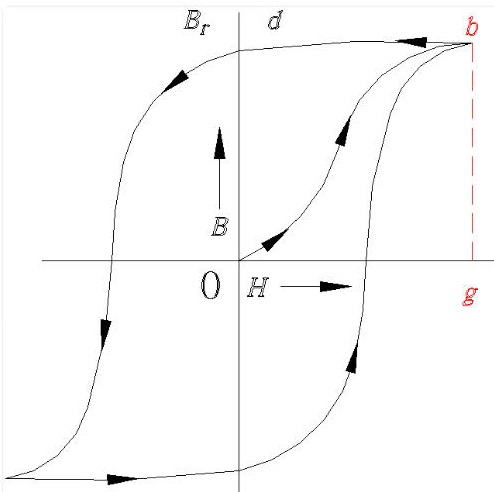
The quantity H is related to the number of ampere-turns imposed divided by the length of the magnetic circuit. The magnetic circuit may be composed of a combination of steel and air paths, and the MMF (or H) divides among the various path segments, based upon the path segment lengths and permeability.
For example, let H in Figure 8 represent the portion of the total MMF that acts on the ferromagnetic material, or steel part. If the steel is initially unmagnetized, it is described by the point labeled 0. There is zero magnetic field (B) with zero imposed MMF (H). If an MMF is imposed equal to the distance 0-g, the material condition is defined by point b. At that point, there is a field in the material proportional to the distance g-b. If the MMF, or excitation field, is then reduced to zero, the material state moves to point d. The MMF is zero, but there is a residual or remnant magnetism (Br) that remains.
If the MMF is successively and repeatedly reversed, the material magnetic states follow the path, referred to as the hysteresis loop, as is shown.
The procedure for demagnetizing (also known as degaussing) a piece of steel to remove its residual magnetism consists of repeatedly applying a reversing, and gradually reduced, MMF. The effect is illustrated in Figure 9.
Figure 9: Successive Hysteresis Loops During the Operation
of Demagnetizing a Ferromagnetic Sample

The process produces cyclically diminishing residual field levels and, if done properly, terminates at the origin, which is the point of zero magnetism. That is except for the Earth's magnetism, which cannot be removed by degaussing, its level ranging from zero to ½ gauss in the absence of nearby magnetic structures or deposits.
Some useful equations for calculating magnetic fields are shown in Figure 10. Equations for calculating forces due to magnetic fields are shown in Figure 11, with an example being shown in Figure 12.
Figure 10: Field Equations for Several Simple Configurations
Figure 11: Magnetically Produced Forces
|
A) Force on a Line of Current in a Magnetic Field
|
|
B) Forces Between Two Lines of Current
|
|
C) Forces Between two Steel Faces with Flux Between Them. (B is Assumed to be Uniform)
|
Figure 12: Forces Developed During Demagnetizing
|
|
||||||||||||||||||
Magnetism in Machinery
Magnetism in machinery accounts for many previously unexplained machinery failures. In particular, the deterioration of bearings, seals, gears, couplings and journals has been attributed to electrical currents in machinery. Often, such trains or machinery groupings contain no components with electrical windings or intended magnetism, i.e., no motors or generators.
Since the turn of the century, manufacturers of electrical equipment have recognized and protected against the effects of electrical shaft currents. Bearing insulation has customarily been utilized for such purposes.
Only since the mid-1970's has the need for protective measures on totally mechanical systems been fully realized. The evolution of turbine and compressor systems towards high speeds and massive frames is acknowledged as the cause for a new source of trouble from magnetic fields.
An electrical generator converts mechanical power to electrical power through magnetic fields. A conventional generator rotor is essentially a magnet that is rotated in such a manner that its magnetic field flux passes through coils of windings. Propitious placement of the coils in slots and other design features result in the conversion of mechanical energy to electrical energy. This produces electrical voltage and power in the windings that is then delivered to the electrical load or power system.
A turbine, compressor, or any other rotating machine that is magnetized behaves much the same way. The magnetic steel parts provide a magnetic circuit, and are also electrically conducting so that voltages are generated, producing localized eddy currents and circulating currents. These currents will be either alternating or direct, and can spark or discharge across gaps and interfaces, producing sparking with frosting, spark tracks, and, in the extreme, welding. They can cause increased temperatures and inflict or initiate severe damage.
The generator action occurs as a result of relative movement between the magnet and the "conductors." Hence, either the frame of a machine or the rotor can be magnetized, and the same action exists when relative motion occurs between the rotating and stationary parts.
The magnetic field density in the air gap of assembled and operating motors and generators is designed to be in the order of 7,000 to 9,000 gauss. These fields are capable of generating from watts to megawatts of electrical power, depending upon the speed and size of the generator.
The field levels due to residual magnetism in turbomachinery occur not from design but from manufacturing, testing, and environmental causes. They have been measured at the surface and in gaps of disassembled parts of a machine at levels from 2 gauss to thousands of gauss. These increase significantly in the assembled machine where the magnetic material provides a good closed path for the magnetism and the air gaps between parts are reduced considerably. This combination can set up conditions for generation of notable stray voltages and the circulation of damaging currents.
There are a number of ways in which steel machinery parts can become magnetized. Placing a part in a strong magnetic field can leave substantial residual magnetism. Mechanical shock and high stressing of some materials can also initiate a residual field.
Some methods creating circular residual magnetism consists of electrical current passing through components. In increasing order of their effect, following are the known examples:
1) Direct current axially through the shaft produces circular magnetism in the shaft. Two obvious sources for this current and circular magnetism are:
- Intentionally imposed high axial current magnetizing to conduct magnetic particle inspection
- Imposition of shaft axially oriented DC current of a synchronous machine, as a result of rotor winding ground fault or short circuit.
2) Electric system faults involving rectified supplies
3) Lightning, discharges, which, separately are credited with causing bearing and also be insidious sources in magnetization of shafts.
The use of electrical welders and heaters on pipes and other parts is common and, if not used properly, will induce residual magnetism.
Items that have been subjected to magnetic particle inspection often retain residual magnetism because of insufficient or improper demagnetizing following the test.
Components that have come in contact with magnetic chucks and magnetic bases often display multiple adjacent poles of a residual field.
Field Measurement and Demagnetizing
Magnetic fields are measured with devices called gaussmeters. As the name implies, these meters measure magnetic flux density in units of gauss. Most meters utilize a probe that works on the "Hall Effect." This type of probe utilizes high frequency currents in its semiconductor chip to produce a characteristic proportional to the magnetic field. Usually, only the very tip of the probe is field sensitive.
Fields that pass perpendicular to the face of the Hall Effect semiconductor are measured. The Hall Effect probe performs expertly in measuring direct (DC) magnetic fields. Its accuracy, and the interpretation of just what is being read if it is employed for measuring alternating (AC) fields, is uncertain and questionable.
Reliable AC gauss or milligauss measurements are usually obtained employing separate circuitry in the gaussmeter, and a different probe encompassing an AC fields sensor coil. It can be used on operating machines or in environments containing alternating fields.
Magnetic fields are directional, being "North" at one end and "South" at the other. Hall Effect probes are directionally sensitive. If the probe is flipped over, a reverse reading is indicated, consistent with sensing either a North or South pole. With digital metering, the sign of the field is automatically indicated (+ or -). Analog meters with a zero center scale will read to the left or right of zero. Keeping one side of the probe (such as the side with the calibration number) always facing away from the object being measured and calling it a North pole when the meter reads positive, establishes a convention for locating North and South poles, and the orientation and path of the magnetism that is creating the poles.
This arbitrary choice for a North pole may be opposite from the established convention; however, it is fully adequate in locating magnetic circuits and their magnetizing forces for purposes of degaussing. Should agreement with established convention on polarity identification be important, the North pole side of an identified reference magnet may be utilized for determining which outward-facing side of the Hall Effect probe produces a positive magnetism reading, which should be labeled North.
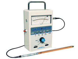
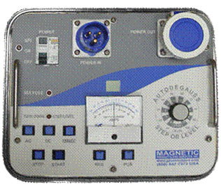
A good gaussmeter has a calibration means to verify proper probe calibration, as well as a zeroing adjustment. The zeroing procedure requires that the probe be temporarily inserted in a "zero gauss chamber." These small chambers shield out stray fields, including the Earth's field, so that a true zero field is realized. This means that strong local field zones can be overlooked. Shown below in Figure 13 are two of MPS’ Gauss Meter offerings.
|
The Original MPS Gaussometer (below) with Auto Ranging and Intuitive Analog Display |
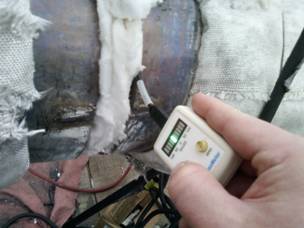
The MPS Pocket Gaussmeter-BarGraph(below) – LED Display: Red=No Weld, Yellow=Possible to Weld, Green=Good to Weld! |
|
|
|
Small, hand-held compass-type "tradeshow giveaways" are often used by maintenance personnel for rough checking of a part or an assembly, while still operational. Experience has demonstrated that these indicators can be grossly inaccurate and prone to breakage and cannot reliably achieve proper orientation and position.
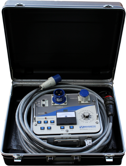
The hardware used for degaussing consists of a power supply and electrical coils that are used to generate magnetic fields. The power supply should have the capability of producing AC or DC output. In the DC mode, a reversing means is necessary to facilitate the downcycling operation. The MPS Auto Degauss System is shown in Figure 14 below.
Output capacities should range up to at least 15,000 ampere-turns and even higher field strengths can be achieved with multiple cable configurations. The coils must be properly sized for the output current, to avoid overheating the insulation. Strong fields can be obtained with a few turns carrying high currents, or many turns carrying low current. The field of the coils is directly proportional to the product of the number of turns and the current (see Figure 10).
|
Figure 14: The Auto Degauss System
|
Auto Degauss in Carrying Case with Degaussing Cable
|
Degaussing units usually have a knob for manually adjusting the output current value, or the starting level for automatic downcycling. When AC output is utilized, the field is inherently reversing at the AC electrical line frequency (50 Hz or 60 Hz). For large or massive components, the high frequency reversing produced in the AC mode can generate surface eddy currents that inhibit penetration of the flux into the part. In these instances, the slower reversing DC technique is required. Units with fully automatic downcycling are the best in meeting this requirement. To use these devices, the coils need to be oriented about the part to be degaussed, the initial power level set and the start cycle button pushed. The degauss cycle is then automatically activated.
For small parts or parts with thin walls, a standard magnetic tape eraser may be effective if employed properly. These devices produce very strong local fields.
Measurement Techniques - At Standstill
The process of measuring magnetic fields requires careful judgment as to where the most meaningful readings can be obtained. On fully assembled machines, the pickup site selections are somewhat restricted. The most critical zones are generally those involving close clearances between rotating and stationary members. Hence, measurements around bearings and seals should be obtained whenever possible. Readings on shaft ends, coupling hubs, gear teeth, foot mountings and pipe flanges are also important.
Where shaft proximity sensors are located, magnetic levels in the areas embraced by the sensor zones should be measured and recorded. Erroneous sensor signals may occur due to magnetic poles or excessive magnetism along the sensor track. This is usually first noticed when performing electrical runout readings at slow roll. Sometimes the sensor manufacturer's application will specify magnetism limits, which must not be exceeded.
Magnetic field levels are best measured with the machinery not operating. The gaussmeter is then used in the DC mode to read static field levels. It should be realized that the field levels can change as the machinery is disassembled because of the alteration in the flux paths. For instance, when a coupling is removed, the adjacent bearing magnetic field levels may increase or decrease. Should it be desirable to investigate the as-assembled magnetism, it is best to perform as little disassembly as possible before making the field readings, so that the measured levels are representative of the operating conditions prior to the shutdown.
As may be noted in the following section, a more useful practice is to conduct magnetic reading surveys on fully disassembled parts, recording readings taken before and after degaussing. Then as assembly takes place, magnetism should be measured on new and reworked parts as they are assembled, and of the assemblies themselves, especially in critical areas such as bearings, seals, gears, etc. High magnetism under these conditions may require downcycling degaussing to achieve acceptable levels.
The practice used in recording and reporting magnetism levels is important in organizing the survey and degaussing activites. A method has been found that is efficient and effective that has been used successfully over the years. This is to first conduct a cursory survey to learn if levels exceed the maximum acceptable magnetism values. If not, then degaussing and a tabulation of magnetic readings may not be necessary. An exception is full circle rings, such as barrel compressor housings and end caps, where captured magnetism closes upon itself and thus does not project to the surface where it can be measured. If shaft current problems are occurring or there is the least suspicion that there is captured magnetism, then low level auto-downcycling should be conducted.
After the cursory survey, it should be decided if the part and its magnetism justify constructing a drawing onto which magnetic readings are to be recorded, or if a tabular form will suffice. In either case, the before and after degauss readings should be written, the latter being designated by encircling or otherwise identifying them. Average and peak values should be recorded, as should the polarities and characteristics of the fields, and whether or not there are localized magnetic poles.
The as-found listing of readings is of inestimable value in selecting the demagnetizing coil placement, and the controller settings and operation. A table of limiting magnetism values that has been developed MPS Gaussbuster Engineer’s many years of experience with close to 1000 turbomachinery installations, is shown below.
Field levels in bearings and seal areas are usually not directly measurable on assemblies as the probe dimensions prohibit insertion between members and in close clearances. The usual approach is to place the probe as close as possible to these zones. It is important to realize that the measured field levels are only fringing values, which can be considerably lower than the actual levels inside the assembly. There is no known method of directly measuring the field levels in solid parts. The internal flux levels are calculated or estimated on the basis of measured values on the boundaries. It is known that assembled unit magnetism levels increase by hundreds or thousands of times the measured open-air values.
Many ferromagnetic materials have permeabilities that vary with field intensities, even at low levels. Hence, there are generally substantial variations of flux density within the these materials. These variations are usually further promoted by geometrical variations of parts and assemblies.
Measurement Techniques - When Operating
By far the greatest amount of information on magnetism and shaft currents in an operating unit is obtained by measuring shaft voltages and currents, utilizing shaft grounding or voltage sensing devices and monitors. Shaft contact devices are intended to ground the shaft, bypassing shaft currents and preventing them from flowing and damaging the bearings, seals and gears, etc. In the past, little attention was paid to the design and performance of grounding devices with the consequence that various amounts of damage occurred, sometimes causing forced outages. Often, the grounding current is passed to the casing or housing directly, with no means to intercept it for measurement and monitoring. Grounding devices employed are often not reliable in a hostile environment. Today, a variety of shaft grounding devices and monitoring equipment are available for protecting critical components and monitoring their performance. Suitable monitors are shown below in Figure 16.
It is a good idea to perform shaft voltage and current tests, utilizing instruments intended for the purpose. Measurements should be made at strategic shaft locations before selection and installation of shaft contact devices. Such tests are useful in showing the character and power delivery capability of the shaft voltages and in determining whether the voltage is static or electromagnetic in nature. While accessibility to the shaft for measurements is often limited, it is usually possible to gain access at one or more locations for testing.
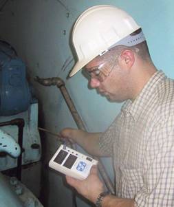
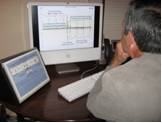
Figure 15: MPS Gaussbuster Engineer performing Shaft Voltage Testing.
|
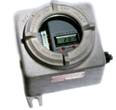
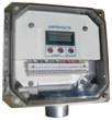
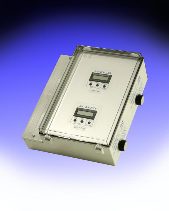
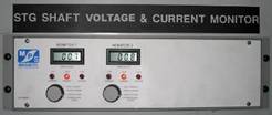
Figure 16: Voltage Current Monitoring Systems Available from MPS: |
|||
|
Single Unit Solutions Explosion proof VCM-EEor
Non- Explosion Proof VCM-EN.
Dual Unit Solution for Turbine Generators VCM-ENSII
Optionally, VCM-ENSII Units can be configured to handle the monitoring of two Turbines, or two Generators in close proximity.
19” Rack Mount Solutions
MPS Shaft Voltage Current Monitors will operate with
most Vendor’s Shaft Grounding or Voltage Sensing Devices.
The only requirement is that the grounding
current device needs to be insulated to provide proper signals to the MPS VCM-E’s. |
|
|
|
If shaft currents from multiple causes occur simultaneously, the trace could be difficult to analyze and multiple considerations may be necessary. MPS Gaussbuster Engineers special in analysis of Shaft Current and Voltage Profiles and determination of root causes of Stray Shaft Currents. The presence of electromagnetic causes dictates that safe and reliable performance can only be assured by conducting a thorough degaussing of the machine and its components Once preferable shaft contact device locations are established, permanent installation, along with accurate and reliable voltage-current monitors, should be made.
When a magnetized piece of machinery is operating, its magnetic field may alternate or pulsate. These can be measured with the MPS Gaussometer switched to the AC mode. Another method consists of using a magnetic sensing "telephone" type pickup connected to a data storage instrument or linear tape recorder. The data can then be analyzed for magnitude and frequency content using spectral analyzers.
Of the several attempts at developing reliable telephone pick-up recordings and AC gaussmeter profiles, none are known to have been continued and trended sufficiently to evaluate their effectiveness. Possibly this is because of the great amount of expense and complication involved in taking, analyzing and deciphering the data.
Accurate predictive and preventative maintenance is the objective of ongoing monitoring of operating performance. As such, it is important that changes be detected and analyzed reliably. This holds for both shaft voltage and current measurements as well as DC and AC magnetic measurements. So long as the same hardware and settings are used at the same locations under controlled load and speed conditions, the same recorded patterns should be present, and changes in the "signatures" can be noted and interpreted. With some experience, the onset of troublesome fields may be detected from shaft voltage and magnetic signatures.
Demagnetizing Techniques
Demagnetizing of equipment requires many considerations and experience in the various techniques and their value and probability of success. The discussed examples and techniques are not intended as a handbook for the inexperienced. If additional information is required, please feel free to contact the Gaussbuster Engineers.
Demagnetizing of turbines, compressors and other machinery is straightforward, except in special or unusual cases. Reliable, established techniques do not always work in every situation. Additionally, material behavior varies and cannot always be accounted for.
For example, experience in degaussing some large and complex components has proved them to demonstrate a remarkable magnetic resilience. Several coil wrap configurations would be used, all with the same results. The fields could be sharply varied by the application of external fields, but the original or only slightly lesser levels returned with the removal of excitation current.
After repeated auto-downcycling with a fixed coil wrap, the fields suddenly and unaccountably diminished sharply. This magnetic "massaging" technique ultimately paid off. In retrospect, it is reasoned that the demagnetizing coils probably did not encircle the magnetic source exactly, and possibly the magnetized material possessed a "square" or stubborn hysteresis loop characteristic.
It is important to remember that magnetic fields can produce substantial forces. (Some useful equations are shown in Figure 11.) When loose parts are placed near each other in magnetic fields, they can experience large attractive forces that can snap them together. Care should be exercised to avoid damage to fingers or valuable equipment.
As an example of these forces, consider two halves of a bearing housing initially separated by ½ inch (see Figure 12). If the open steel loop is wrapped with a coil producing 4,000 ampere-turns, an air gap density of 1,960 gauss is established (per Figure 10c). The pinching force in the initial position (assuming a gap face area of 10 sq. inches) is 22 pounds at each split. As the two halves pull together, the flux density will increase. With an opening of ¼ inch, the force is near 88 pounds. At 1/8 inch spacing, the pinching force is over 355 pounds at each gap!
Very large forces can be readily created during the demagnetizing process. The forces increase dramatically as the parts come closer together. Loose parts should be suitably clamped or braced prior to applying fields.
Maintenance Recommendations
Many costly outages can be averted by implementing proper maintenance practices. Damaging magnetic fields initially manifest themselves in the form of "frosted" bearings and/or spark tracking on bearings, seals, couplings or gears. Examples of Rotating Machinery Damage is available from MPS.
The exact cause for magnetization is frequently difficult to determine. Welding, electrostatic discharge, the use of magnetic tools or chucks, and improperly degaussed Magnafluxed parts, are all potential sources.
Good maintenance practices require:
1. A thorough visual inspection of bearings, seals, couplings and gears during regular, scheduled shutdowns, for signs of magnetically-induced current damage.
2. Monitoring of the shaft position radially and axially with a proximity probe. This should be continued on a regular basis, since ultimate damage results in loss of babbitt or steel. Often, an increase in bearing temperatures occurs as well.
3. Monitoring shaft currents with an instrument such as MPS VCMs, that will display (or preferably record) accurately and consistently the shaft currents in the grounding cable connected to a shaft grounding device. Notable changes should flag a potential problem.
A plan of action should be formulated based upon the magnitude and significance of the change. Consult MPS Gaussbuster Engineers for Data Analysis Assistance.
4. Checking and maintaining shaft grounding devices on a regular basis to insure their proper performance and grounding of the shaft.
5. Insuring that all welding is performed with the grounding electrode connected as close as possible to the weld area.
6. Checking magnetism with an accurate gaussmeter, such as the MPS Gaussometer, on all new parts for storage or addition to the lineup to insure that they are properly demagnetized before installation. Part specification should include a demagnetization requirement, with acceptable levels not to exceed those listed in the table (above) labeled "Maximum Allowable Residual Magnetic Field Levels" as defined by MPS Gaussbuster Engineers after many years of experience.